How I Built an Orchestrated NL2SQL Pipeline That Scales with Complexity
Natural language to SQL is one of those widely applicable problems that has not yet been solved with AI. On BIRD, the hardest public text-to-SQL benchmark, state-of-the-art single-pass systems top out around 75% execution accuracy. Human experts score 92.96%. The gap sits almost entirely on complex, multi-join, domain-rich questions where schema ambiguity and missing literals trip up every model.
This post walks through scale-analytics, a pipeline I built that reaches 89.67% execution accuracy on the test set by combining three axes of compute scaling — parallel synthesis, iterative refinement, and tournament selection — into a single orchestrated system. The goal was a production-grade design: observable, testable, model-agnostic, and runnable without proprietary RL-trained checkpoints.
The Core Insight: Scaling Compute, Not Parameters
This is a restatement of Sutton’s Bitter Lesson applied to inference: given a fixed model budget, the best lever is more compute at query time, not a bigger model or better prompts. Three scaling axes compound:
- Parallel (width): generate many SQL candidates with diverse strategies and temperatures.
- Sequential (depth): iteratively refine each candidate — fix syntax errors, then semantically revise.
- Internal (quality): use RL-trained models that reason longer per token rather than stopping at the first plausible answer.
The architecture translates these three axes into four layers.
Architecture Overview: L0 to L3
L0 (offline, per-database)
  |
  +--> Light Schema  (markdown table + column descriptions)
  +--> DDL Schema    (CREATE TABLE for code-specialised models)
  +--> Cell Vector Store  (Chroma, all-MiniLM-L6-v2, one per DB)
  +--> Example Vector Store  (Chroma, question skeleton -> sql)
  +--> BM25 Index    (lexical fallback)

L1 (online, per query) -- Task Understanding
  KeywordSkeletonExtractor --> CellRetriever || ExampleRetriever

L2 (online) -- SQL Generation Scaling
  ReasoningGenerator || ICLGenerator x 3 strategies
  --> ExecutionBucketer --> SQLFixer (syntax) --> CritiqueAgent --> SQLRevisor (semantic)
  * critique-conditioned re-synthesis (up to 2 passes)

L3 (online) -- SQL Selection Scaling
  ExecutionBucketer --> TournamentArbiter --> ReasoningSelector
  --> Final SQL
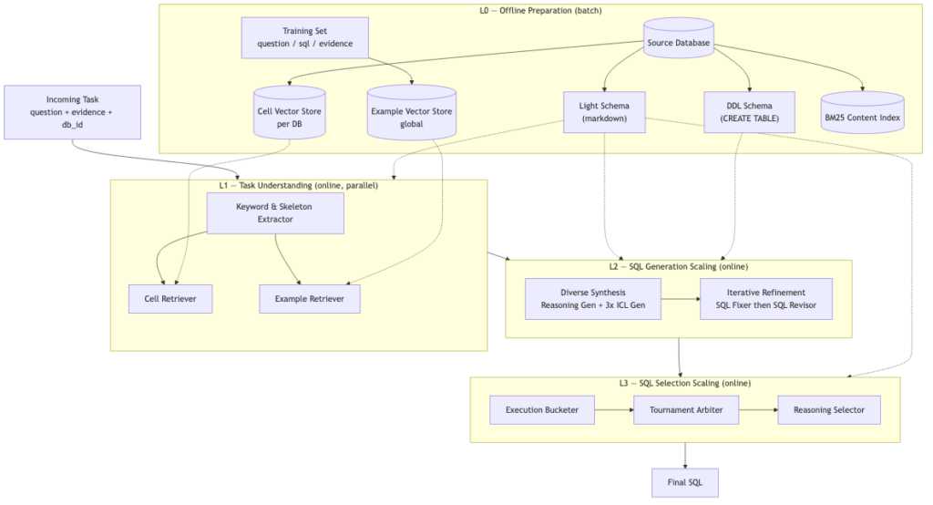
L0 runs once when database fields are updated. L1–L3 run on every incoming query. The total LLM call count per query is around fifteen in the default configuration — expensive, but the pipeline is designed to scale down for simple questions via a difficulty router that reduces k_icl and disables the tournament when the question is straightforward.
L1: Task Understanding
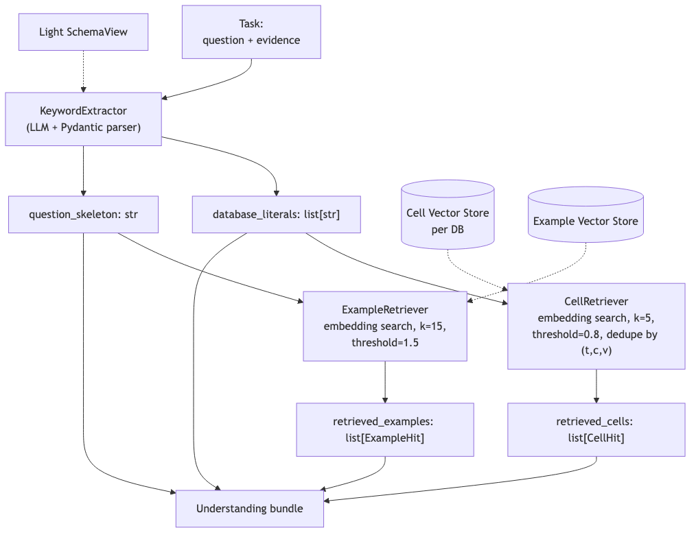
The first online stage extracts two things from the incoming question: database literals (exact cell values the SQL will need to match verbatim) and a question skeleton (a structural abstraction used to find similar few-shot examples).
These run in parallel via LangGraph’s Send primitive:
KeywordSkeletonExtractor (LLM, Gemini Flash T=0.2)
         |
         +--> literals --> CellRetriever (k=5, cosine threshold 0.8)
         `--> skeleton --> ExampleRetriever (k=15, threshold 1.5)
Cell retrieval searches a per-DB Chroma collection built from TEXT columns in the source database, filtered to exclude primary keys, IDs, emails, and strings over 256 characters. Example retrieval searches a global collection of training-set question skeletons to find structurally similar past questions with known-correct SQL.
Both retrievers return typed Pydantic objects (CellHit, ExampleHit) that the downstream generators consume directly — no string concatenation, no ad-hoc dicts.
L2: SQL Generation Scaling
This is where the diversity-then-refinement strategy plays out.
Diverse Synthesis
Two generator families run in parallel, each with a different schema view and a different prompting approach:
ReasoningGenerator — sees the DDL schema (CREATE TABLE with inline comments), no examples. Uses chain-of-thought inside <think>…</think> tags, then emits SQL inside <sql>…</sql>. Designed to slot in RL-trained reasoning checkpoints when available; falls back to DeepSeek-Coder-V2 or GPT-5 at high effort today.
ICLGenerator — sees the light markdown schema plus retrieved few-shot examples. Runs three sub-prompts in parallel to maximise diversity:
- Direct: few-shot SQL completion.
- Chain-of-Thought: reason in natural language, then emit SQL.
- Question Decomposition: split into sub-questions, solve bottom-up, compose the final SQL.
Each of these generators outputs the commented SQL along with the reasoning in bullet points. Default configuration: 2 reasoning candidates + 2 × 3 ICL candidates = 8 total. Every candidate is executed immediately in the sandbox and tagged with its ExecutionResult.
Iterative Refinement
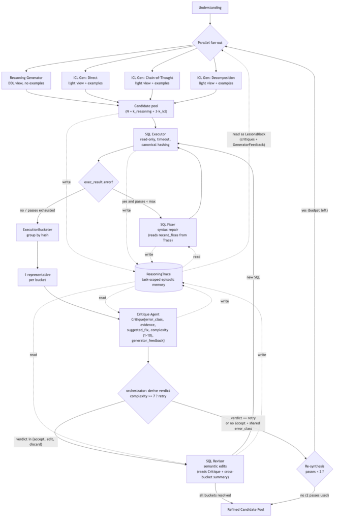
The refinement loop composes three agentic patterns so it learns within a single query from every generator’s reasoning, rather than treating each candidate as an independent draft:
- Reflection — a dedicated
CritiqueAgentseparates generation from evaluation; structured feedback drives the next edit. - Memory Management — a task-scoped
ReasoningTraceacts as an episodic scratchpad, recording every generator’s rationale, execution result, and critique for the duration of one query. - Learning and Adaptation — when the critique signals a framing problem that revision alone can’t fix, the orchestrator re-invokes the generators with accumulated lessons injected into their prompts.
The four components of the loop, in order:
ExecutionBucketer (no LLM) groups all candidates by ExecutionResult.hash. Candidates with errors or zero rows are flagged suspicious. Bucket metadata — size, producer mix, mean rationale length — is written to ReasoningTrace so downstream agents know which generators agreed.
SQLFixer (conditional) repairs candidates that errored. It reads ReasoningTrace.recent_fixes(producer) to avoid repeating a repair strategy that already failed on a sibling candidate from the same generator. Bounded at 2 passes; failed candidates are dropped from the tournament but kept in the trace.
CritiqueAgent (new) runs once per non-error bucket, before the revisor. It reads the bucket representative, its reasoning trace, and the rationales of every other generator — so it can contrast hypotheses, not just evaluate one candidate in isolation. It emits a typed Critique with:
error_class— a closed enum (wrong_join,missing_filter,wrong_aggregation,value_mismatch,evidence_ignored,other) so critiques are aggregatable across buckets and queries.complexity— an integer 1–10 rating of how convoluted the reasoning required to answer the question is, based on the spread of generator rationales and the bucket representative’s structure. Anything ? 7 means editing alone is unlikely to converge.suggested_fix— an actionable rewrite hint for the revisor.generator_feedback— corrective material (correctionorwarning) for the generators on a re-synthesis pass, distinct fromsuggested_fixbecause it needs to be generic enough to seed multiple new candidates from different prompting strategies.
The retry verdict is derived by the orchestrator, not chosen by the LLM: if complexity >= 7, the orchestrator forces verdict = "retry" regardless of what the model wrote. This keeps the threshold a single source of truth in code and makes it unambiguously trace-grounded.
SQLRevisor runs on bucket representatives when the verdict is edit. It now receives the Critique (what is wrong) and a cross-bucket summary from ReasoningTrace (what other generators answered instead), so it is no longer reasoning blind about a single candidate. Bounded at 1–2 passes; any new SQL re-enters the loop from execution onward.
Critique-Conditioned Re-Synthesis
After each revisor pass, the orchestrator checks whether re-synthesis is warranted. It triggers a new generation round when either:
- Any bucket’s critique has
complexity >= 7(aretryverdict) — high-complexity questions are where framing errors happen at synthesis time, not editing time. - No bucket was accepted and at least one
error_classis shared across two or more buckets — meaning the generators systematically misread the same aspect of the question.
When triggered, the generators are re-invoked with a LessonsBlock injected into their prompts, assembled from ReasoningTrace:
Avoid: wrong_join — the join through order_items produces duplicate rows.
Prefer: join through orders directly.

## Corrections
- The join must go through orders, not order_items. [all generators]

## Warnings
- Be careful with NULL handling on customer.region. [icl/direct only]
New candidates re-enter the full loop (execution ? bucketing ? critique ? revision). Re-synthesis is capped at 2 passes (resynth_max_passes) and generates k_resynth = max(1, k_icl // 2) candidates per generator per pass. After 2 passes, L3 runs on whatever pool exists — the cap is non-negotiable to prevent reflection-loop runaway.
The ReasoningTrace itself is task-scoped and ephemeral: it lives for the duration of one query and is serialised into the final TaskContext for L3 and post-hoc analysis, but it is not long-term memory. Recurring lessons (distilled (skeleton, error_class, fix) triples) can optionally be written to a cross-task lesson store that augments L1 example retrieval on future queries — but that path is offline and does not affect the serving pipeline’s statefulness invariant.
L3: SQL Selection Scaling
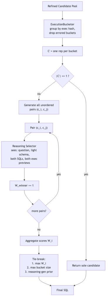
After refinement, you have a pool of candidates grouped by execution result hash. The tournament works like this:
- Take one representative per non-error bucket ? set
C'. - If
|C'| == 1, return it immediately. - Otherwise run pairwise round-robin: for every unordered pair
(c_i, c_j), ask theReasoningSelectorwhich SQL better answers the question. It sees the question, the light schema, both SQL strings, and both execution previews. - Rank by win count. Tie-break: (a) higher win count, (b) larger bucket (more generators agreed), (c) prefer the reasoning generator (empirically higher precision on simple/moderate questions).
Complexity is O(|C'|²) selector calls. In practice |C'| is 2–5 after bucketing, so the tournament costs 1–10 calls.
The Orchestrator: LangGraph as the Graph Runtime
The orchestrator is the only place where scaling lives as code. Agents are stateless; they have no idea about retries, fan-out width, or loop depth. The orchestrator’s ScalingConfig owns all of that:
class ScalingConfig(Frozen):
    k_reasoning: int = 2
    k_icl: int = 2                     # per sub-prompt
    k_resynth: int = 1                 # candidates per generator on re-synthesis (default max(1, k_icl//2))
    fixer_max_passes: int = 2
    refinement_max_passes: int = 1
    resynth_max_passes: int = 2        # critique-conditioned re-synthesis depth
    complexity_retry_threshold: int = 7  # Critique.complexity at or above which verdict is forced to "retry"
    tournament_enabled: bool = True
    global_timeout_s: int = 120
    token_budget: int = 200_000
I chose LangGraph over CrewAI, smolagents, Google ADK, and plain asyncio for one concrete reason: the pipeline’s structure — two fan-outs, two bounded loops, one tournament — maps directly onto LangGraph primitives. The Send primitive expresses per-candidate execution, per-bucket revision, and per-pair selector calls as first-class graph nodes rather than hand-rolled asyncio.gather blocks. Conditional edges express exec_result.error? ? fixer and refinement_passes_left? ? revisor without hand-rolled while loops. Checkpointers give us replay for free.
What we deliberately don’t take from LangGraph: its model wrappers. Every LLM call goes through our own model-adapter, and our AgentEvent schema is the authoritative lineage format — LangSmith and JSONL are sinks, not owners.
Data Contracts: Pydantic Frozen Models
Every type that crosses a module boundary is an immutable Pydantic v2 model. No dicts, no prompt strings, no ad-hoc tuples.
class Frozen(BaseModel):
    model_config = ConfigDict(frozen=True, extra="forbid", str_strip_whitespace=True)

class CandidateSQL(Frozen):
    sql: str
    producer: str                          # "reasoning/T=0.7", "icl/cot/T=1.0"
    rationale: Optional[str] = None
    exec_result: Optional[ExecutionResult] = None
    lineage: list[str] = Field(default_factory=list)  # ["gen", "fix", "revise:pass2"]

class ExecutionResult(Frozen):
    rows: tuple[tuple, ...]
    columns: tuple[str, ...]
    row_count: int = Field(ge=0)
    error: Optional[str] = None
    hash: str
    elapsed_ms: int = Field(ge=0)
frozen=True makes every contract hashable and safe to share across async tasks. extra="forbid" catches typos. ExecutionResult.hash is computed over a canonical form of the result set — sorted rows, normalised timestamps, float rounding to 6 decimal places — so that two syntactically different SQLs that return the same answer collapse into the same bucket.
The Execution Sandbox
Every candidate SQL is executed in a read-only sandbox before any LLM refinement or selection decision. This is load-bearing: bucketing, revision, and tournament selection all depend on the canonical hash.
Read-only enforcement is multi-layered:
- SQLite:
PRAGMA query_only = ON, opened withmode=roURI. - A lightweight AST check rejects
INSERT | UPDATE | DELETE | DROP | ALTER | ATTACHbefore execution reaches the driver. - Write violations raise
ReadOnlyViolationsynchronously; the connection is discarded, not returned to the pool.
The canonicalisation pipeline:
raw rows
  --> sort in-memory (stable tuple comparator; do NOT add ORDER BY to the SQL)
  --> normalise per cell (rstrip strings, round floats to 6dp, ISO-8601 timestamps, null sentinel)
  --> BLAKE2b hash over canonical JSON
Error results get an ERR: prefixed hash so they can never hash-collide with a successful result, and identical syntax errors across multiple candidates collapse into the same error bucket.
Observability: Three-Surface Tracing
Every agent call emits a typed AgentEvent following OpenTelemetry GenAI semantic conventions. Events are tagged with one of three surfaces:
| Surface | What it measures | Example agents |
|---|---|---|
cognitive | Plan quality, reasoning correctness | Keyword extractor, generators, selector |
operational | Tool-call reliability | SQL executor, fixer |
contextual | Retrieval precision | Cell retriever, example retriever |
The evaluation harness derives per-surface metrics from this stream: Plan Adherence Rate, Tool Call Success Rate, Retrieval Precision, and Critic Adherence Rate (how often the Revisor actually adopts its own critique).
The Revisor’s reflection loop is a first-class event:
async with tracer.span("l2.sql_revisor", surface="cognitive", node="l2.revise") as span:
    verdict = await self._critique(candidate)
    await tracer.critique(
        "l2.sql_revisor",
        RevisionDelta(
            before_hash=candidate.exec_result.hash,
            after_hash=new_result.hash,
            verdict="revise",
            rationale="...",
        ),
    )
    span.set_output(revised_candidate)
This design lets you compute Critic Adherence Rate offline: for every case where the critique agent said “this needs a change,” did the new candidate actually produce a different result?
Events fan out to LangSmith (default) and a local JSONL file in parallel. If LangSmith is unreachable, the pipeline continues with the JSONL sink and logs a single warning.
DSPy for Prompt Compilation
Agents that the pipeline actually cares about optimising — the keyword extractor, the three ICL generator sub-prompts, the CritiqueAgent, the revisor, and the selector — are expressed as DSPy Signatures compiled against execution-grounded metrics.
The Revisor’s compilation metric is approximately:
def revisor_metric(example, pred, trace=None):
    result = sandbox.execute(pred.sql, db_id=example.db_id)
    if result.hash == example.gold_hash:
        return 1.0
    elif result.error is None:
        return 0.1
    return 0.0
The metric mirrors the same execution-grounded reward used to train RL-tuned reasoning models. When a stronger checkpoint becomes available, it replaces the compiled prompt behind the same DSPy Signature with zero orchestration changes — the signature is the contract, and either side (compiled prompt or RL model) can fulfill it.
Graceful Degradation
The pipeline fails hard in exactly one scenario: every generator produced zero candidates. Otherwise degradation is priority-ordered and monotonic:
KeywordSkeletonExtractorfails –> continue with emptyUnderstanding.CellRetrieverorExampleRetrieverfails –> continue with empty list.- One ICL sub-prompt fails –> continue with remaining generators.
SQLFixer/SQLRevisorfails –> skip that pass, keep pre-refinement candidates.ReasoningSelectorfails mid-tournament –> fall back to majority vote over bucket sizes.- Budget or timeout exceeded –> return best-so-far candidate tagged
degraded=True.
Every degradation fires a DecisionEvent with a label, confidence, and feature dict. The evaluation harness computes degraded_rate from the trace — so you can see whether degraded runs score proportionally worse and by how much.
Evaluation
The evaluation harness runs on a proprietary set of commonly asked questions in the healthcare domain about claims data. Primary metric is execution accuracy — does the candidate SQL produce the same result set as the gold SQL? Secondary is reward-based valid efficiency score, which weights correct queries by execution-time ratio vs gold.
The ablation table covers: drop the reasoning generator, drop ICL, drop the tournament (? self-consistency), drop refinement. Any fork of this codebase can compare directly.
References
- Sutton (2019). The Bitter Lesson. incompleteideas.net